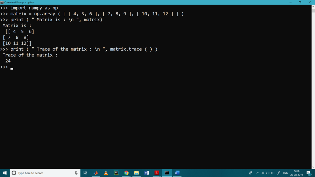
Trace of a Matrix Calculations

Trace of a Matrix is the sum of diagonal elements of the Matrix.

>>> import numpy as np

>>> matrix = np.array ( [ [ 4, 5, 6 ], [ 7, 8, 9 ], [ 10, 11, 12 ] ] )

>>> print ( ” Matrix is : \n “, matrix)

 Matrix is :

  [[ 4  5  6]

 [ 7  8  9]

 [10 11 12]]

>>> print ( ” Trace of the matrix : \n “, matrix.trace ( ) )

 Trace of the matrix :

  24

>>> 

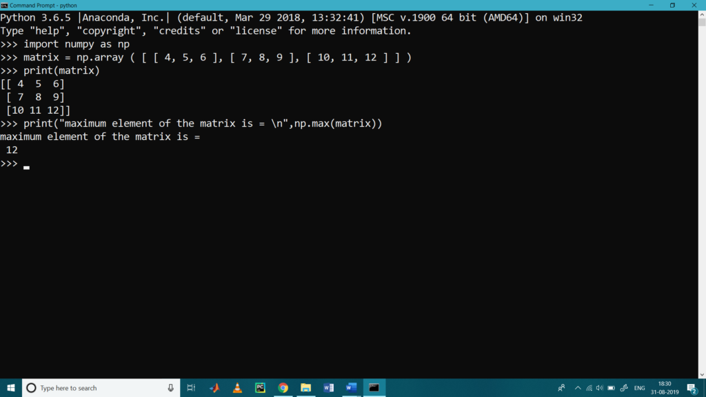
Finding Maximum Values in Matrix

To find maximum value from the matrix we used max ().

>>> import numpy as np

>>> matrix = np.array ( [ [ 4, 5, 6 ], [ 7, 8, 9 ], [ 10, 11, 12 ] ] )

>>> print(matrix)

[[ 4  5  6]

 [ 7  8  9]

 [10 11 12]]

>>> print(“maximum element of the matrix is = \n”,np.max(matrix))

maximum element of the matrix is =

 12

Learn Python with our Expert Trainers

Finding Minimum Values in Matrix

To find minimum value from the matrix we used min ().

>>> import numpy as np

>>> matrix = np.array ( [ [ 4, 5, 6 ], [ 7, 8, 9 ], [ 10, 11, 12 ] ] )

>>> print ( matrix )

[[ 4  5  6]

 [ 7  8  9]

 [10 11 12]]

>>> print  ( “minimum element of the matrix is = \n”, np.min(matrix) )

minimum element of the matrix is =

 4

>>> 

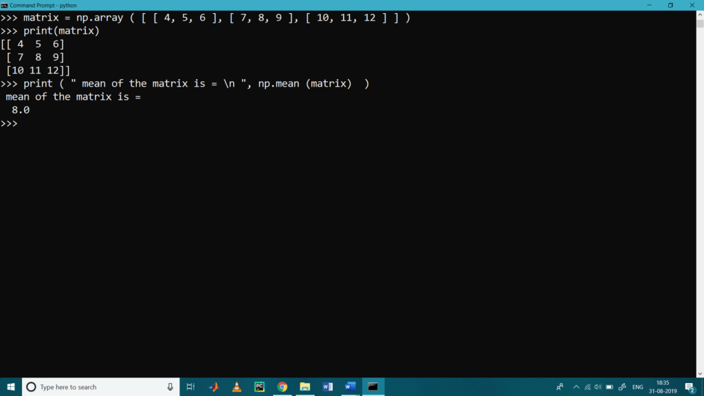
Average Calculation

To calculate average of all the element present in the matrix we use mean()

>>> import numpy as np

>>> matrix = np.array ( [ [ 4, 5, 6 ], [ 7, 8, 9 ], [ 10, 11, 12 ] ] )

>>> print(matrix)

[[ 4  5  6]

 [ 7  8  9]

 [10 11 12]]

>>> print ( ” mean of the matrix is = \n “, np.mean (matrix)  )

 mean of the matrix is =

  8.0

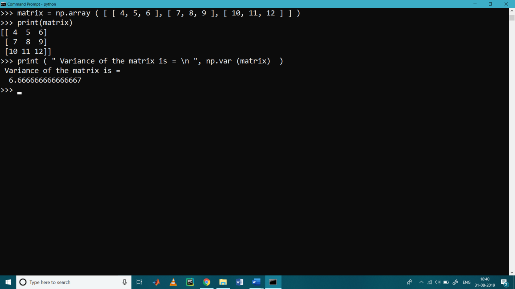
Variance Calculation

To calculate the variance of the matrix we used var()

>>> import numpy as np

>>> matrix = np.array ( [ [ 4, 5, 6 ], [ 7, 8, 9 ], [ 10, 11, 12 ] ] )

>>> print(matrix)

[[ 4  5  6]

 [ 7  8  9]

 [10 11 12]]

>>> print ( ” Variance of the matrix is = \n “, np.var (matrix)  )

 Variance of the matrix is =

  6.666666666666667

>>> 

Standard deviation Calculation

To calculate the variance of the matrix we used std()

>>> import numpy as np

>>> matrix = np.array ( [ [ 4, 5, 6 ], [ 7, 8, 9 ], [ 10, 11, 12 ] ] )

>>> print(matrix)

[[ 4  5  6]

 [ 7  8  9]

 [10 11 12]]

>>> print ( ” Standard Deviation of the matrix is = \n “, np.std (matrix)  )

 Standard Deviation of the matrix is =

  2.581988897471611

>>> 

Use of numpy.linalg

The numpy.linalg library is used  calculates the determinant of the input matrix, rank of the matrix, Eigenvalues and Eigenvectors of the matrix

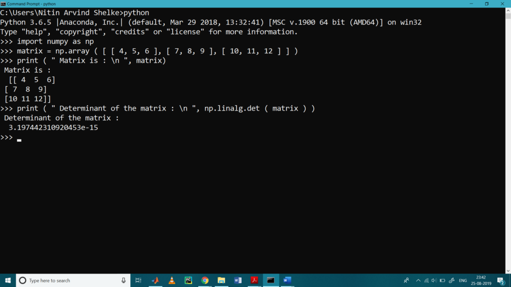
1. Determinant Calculation

np.linalg.det is used to find the determinant of matrix.

>>> import numpy as np

>>> matrix = np.array ( [ [ 4, 5, 6 ], [ 7, 8, 9 ], [ 10, 11, 12 ] ] )

>>> print ( ” Matrix is : \n “, matrix)

 Matrix is :

  [[ 4  5  6]

 [ 7  8  9]

 [10 11 12]]

>>> print ( ” Determinant of the matrix : \n “, np.linalg.det ( matrix ) )

 Determinant of the matrix :

  3.197442310920453e-15

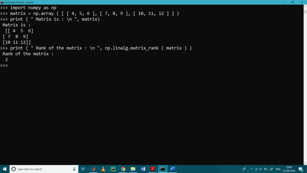
• Rank of a Matrix

The rank of a matrix rows (columns) is the maximum number of linearly independent rows (columns) of this matrix, that is count of number of non-zero rows. np.linalg.rank is used to find the rank of the matrix.

>>> import numpy as np

>>> matrix = np.array ( [ [ 4, 5, 6 ], [ 7, 8, 9 ], [ 10, 11, 12 ] ] )

>>> print ( ” Matrix is : \n “, matrix)

 Matrix is :

  [[ 4  5  6]

 [ 7  8  9]

 [10 11 12]]

>>> print ( ” Rank of the matrix : \n “, np.linalg.matrix_rank ( matrix ) )

 Rank of the matrix :

  2

>>> 

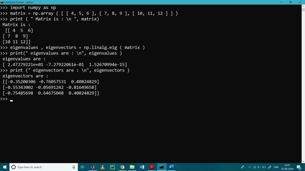
• Eigenvalues and Eigenvectors

Eigenvectors are widely used in Machine Learning image processing. Eigenvectors are vectors that when that transformation is applied, change only in scale (not direction). np.linalg.eig() is used to find the eigen values and eigen vectors of the matrix.

>>> import numpy as np

>>> matrix = np.array ( [ [ 4, 5, 6 ], [ 7, 8, 9 ], [ 10, 11, 12 ] ] )

>>> print ( ” Matrix is : \n “, matrix)

 Matrix is :

  [[ 4  5  6]

 [ 7  8  9]

 [10 11 12]]

>>> eigenvalues , eigenvectors = np.linalg.eig ( matrix )

>>> print(” eigenvalues are : \n”, eigenvalues )

 eigenvalues are :

 [ 2.47279221e+01 -7.27922061e-01  1.52670994e-15]

>>> print (” eigenvectors are : \n”, eigenvectors )

 eigenvectors are :

 [[-0.35200306 -0.76057531  0.40824829]

 [-0.55343002 -0.05691242 -0.81649658]

 [-0.75485698  0.64675048  0.40824829]]

>>> 

Use of numpy.matlib

NumPy package contains a Matrix library numpy.matlib. Some of the useful function included in matlib are as follows.

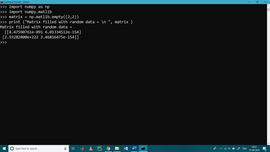
1. matlib.empty()

This function returns a new matrix filled with the random data.

>>> import numpy as np

>>> import numpy.matlib

>>> matrix = np.matlib.empty((2,2))

>>> print (“Matrix filled with random data = \n “, matrix )

Matrix filled with random data =

  [[4.47590761e-091 6.01334512e-154]

 [2.93282800e+222 2.46816475e-154]]

>>> 

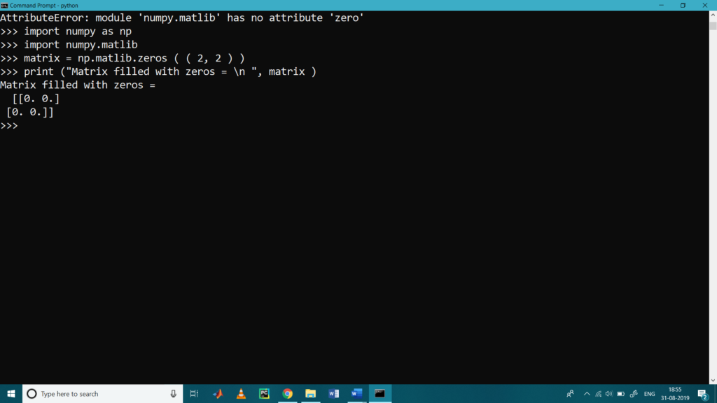
• matlib.zeros()

It is used to filled matrix with zero.

>>> import numpy as np

>>> import numpy.matlib

>>> matrix = np.matlib.zeros ( ( 2, 2 ) )

>>> print (“Matrix filled with zeros = \n “, matrix )

Matrix filled with zeros =

  [[0. 0.]

 [0. 0.]]

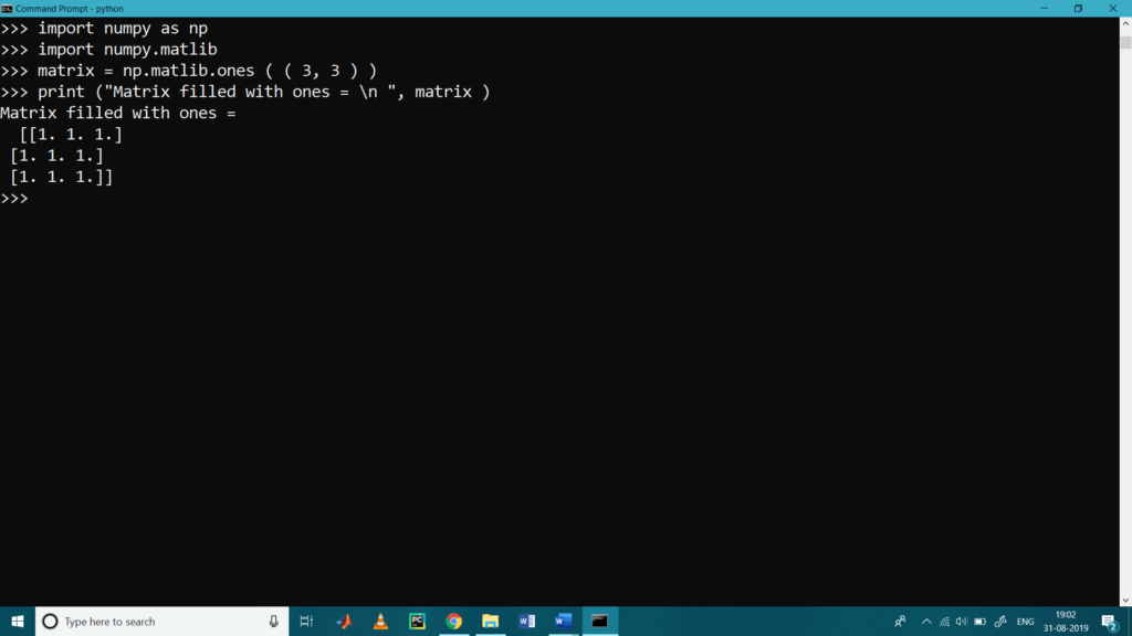
• matlib.ones()

It is used to filled the matrix with ones.

>>> import numpy as np

>>> import numpy.matlib

>>> matrix = np.matlib.ones ( ( 3, 3 ) )

>>> print (“Matrix filled with ones = \n “, matrix )

Matrix filled with ones =

  [[1. 1. 1.]

 [1. 1. 1.]

 [1. 1. 1.]]

>>> 

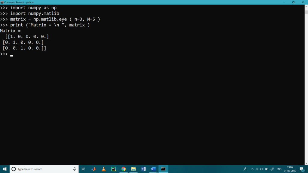
• matlib.eye()

This function returns a matrix with 1 along the diagonal elements and the zeros elsewhere.

>>> import numpy as np

>>> import numpy.matlib

>>> matrix = np.matlib.eye ( n=3, M=5 )

>>> print (“Matrix = \n “, matrix )

Matrix =

  [[1. 0. 0. 0. 0.]

 [0. 1. 0. 0. 0.]

 [0. 0. 1. 0. 0.]]

>>> 

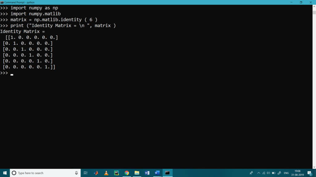
• matlib.identity()

It is similar to eye()and use to obtain the identity matrix (Matric with diagonal element 1)

>>> import numpy as np

>>> import numpy.matlib

>>> matrix = np.matlib.identity ( 6 )

>>> print (“Identity Matrix = \n “, matrix )

Identity Matrix =

  [[1. 0. 0. 0. 0. 0.]

 [0. 1. 0. 0. 0. 0.]

 [0. 0. 1. 0. 0. 0.]

 [0. 0. 0. 1. 0. 0.]

 [0. 0. 0. 0. 1. 0.]

 [0. 0. 0. 0. 0. 1.]]

>>>