NLTK Sentiment Analysis – About NLTK :
- The Natural Language Toolkit, or more commonly NLTK, is a suite of libraries and programs for symbolic and statistical natural language processing (NLP) for English written in the Python programming language.
- It was developed by Steven Bird and Edward Loper in the Department of Computer and Information Science at the University of Pennsylvania.
Sentiment Analysis :
Sentiment Analysis is a branch of computer science, and overlaps heavily with Machine Learning, and Computational Linguistics Sentiment Analysis is the most common text classification tool that analyses an incoming message and tells whether the underlying sentiment is positive, negative our neutral.
It the process of computationally identifying and categorizing opinions expressed in a piece of text, especially in order to determine whether the writer’s attitude towards a particular topic, product, etc. is positive, negative, or neutral.
Sentiment Analysis is a concept of Natural Language Processing and Sometimes referred to as opinion mining, although the emphasis in this case is on extraction

Examples of the sentimental analysis are as follows :
- Is this product review positive or negative?
- Is this customer email satisfied or dissatisfied?
- Based on a sample of tweets, how are people responding to this ad campaign/product release/news item?
- How have bloggers’ attitudes about the president changed since the election?
- The purpose of this Sentiment Analysis is to automatically classify a tweet as a positive or Negative Tweet Sentiment wise
- Given a movie review or a tweet, it can be automatically classified in categories. These categories can be user defined (positive, negative) or whichever classes you want.
- Sentiment Analysis for Brand Monitoring
- Sentiment Analysis for Customer Service
- Sentiment Analysis for Market Research and Analysis

Sample Positive Tweets
- I love this car
- This view is amazing
- I feel great this morning
- I am so excited about the concert
- He is my best friend
Sample Negative Tweets
- I do not like this car
- This view is horrible
- I feel tired this morning
- I am not looking forward to the concert
- He is my enemy
Sentimental Analysis Process
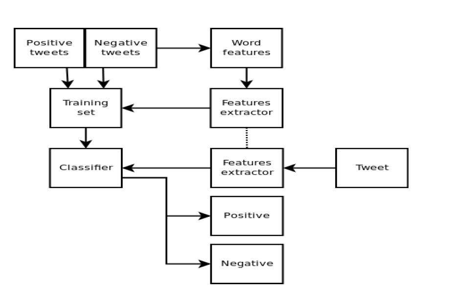
- The list of word features need to be extracted from the tweets.
- It is a list with every distinct word ordered by frequency of appearance.
- The use of Feature Extractor to decide which features are more relevant.
- The one we are going to use returns a dictionary indicating that words are contained in the input passed.
Naive Bayes Classifier
- It uses the prior probability of each label – which is the frequency of each label in the training set and the contribution from each feature.
- In our case, the frequency of each label is the same for ‘positive’ and ‘negative’.
- Word ‘amazing’ appears in 1 of 5 of the positive tweets and none of the negative tweets.
- This means that the likelihood of the ‘positive’ label will be multiplied by 0.2 when this word is seen as part of the input
Sentiment Analysis Example 1 :
Training Data
- This is a good book! Positive
- This is a awesome book! Positive
- This is a bad book! Negative
- This is a terrible book! Negative
Testing Data
- This is a good article
- This is a bad article
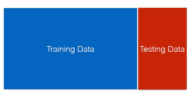
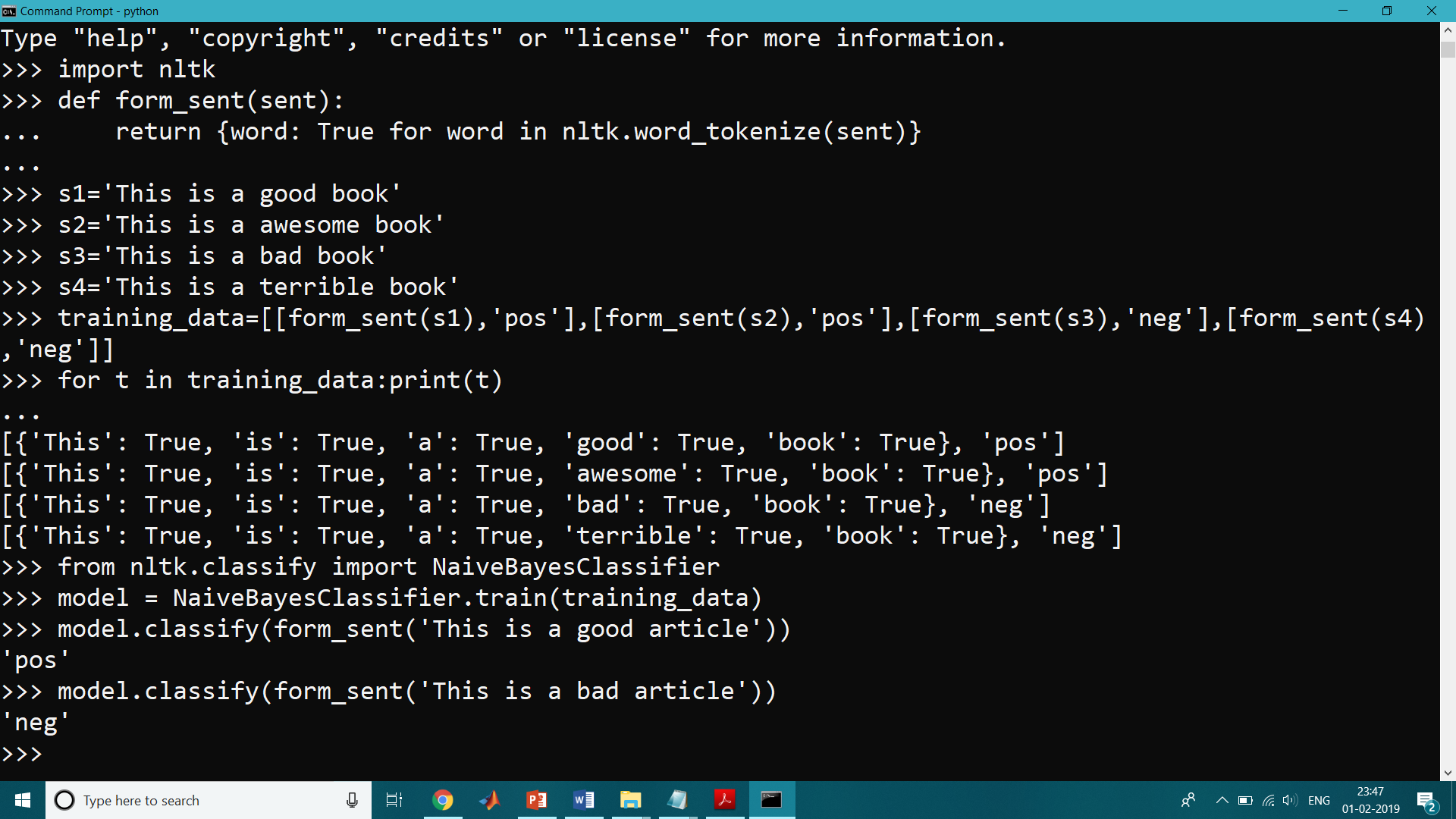
We will train the model with the help of training data by using Naïve Bayes Classifier.
And then test the model on testing data.
>>> def form_sent(sent):

...     return {word: True for word in nltk.word_tokenize(sent)}

...

>>> form_sent("This is a good book")

{'This': True, 'is': True, 'a': True, 'good': True, 'book': True}

>>> s1='This is a good book'

>>> s2='This is a awesome book'

>>> s3='This is a bad book'

>>> s4='This is a terrible book'

>>> training_data=[[form_sent(s1),'pos'],[form_sent(s2),'pos'],[form_sent(s3),'neg'],[form_sent(s4),'neg']]


>>> for t in training_data:print(t)

...

[{'This': True, 'is': True, 'a': True, 'good': True, 'book': True}, 'pos']

[{'This': True, 'is': True, 'a': True, 'awesome': True, 'book': True}, 'pos']

[{'This': True, 'is': True, 'a': True, 'bad': True, 'book': True}, 'neg']

[{'This': True, 'is': True, 'a': True, 'terrible': True, 'book': True}, 'neg']

>>> from nltk.classify import NaiveBayesClassifier

>>> model = NaiveBayesClassifier.train(training_data)

>>> model.classify(form_sent('This is a good article'))

'pos'

>>> model.classify(form_sent('This is a bad article'))

'neg'

>>>
Accuracy
NLTK has a built-in method that computes the accuracy rate of our model:
>>> from nltk.classify.util import accuracy
Sentiment Analysis Example 2 :
Gender Identification: – we know that male and female names have some distinctive characteristics. Generally, Names ending in a, e and i are likely to be female, while names ending in k, o, r, s and t are likely to be male.
We build a classifier to model these differences more precisely.
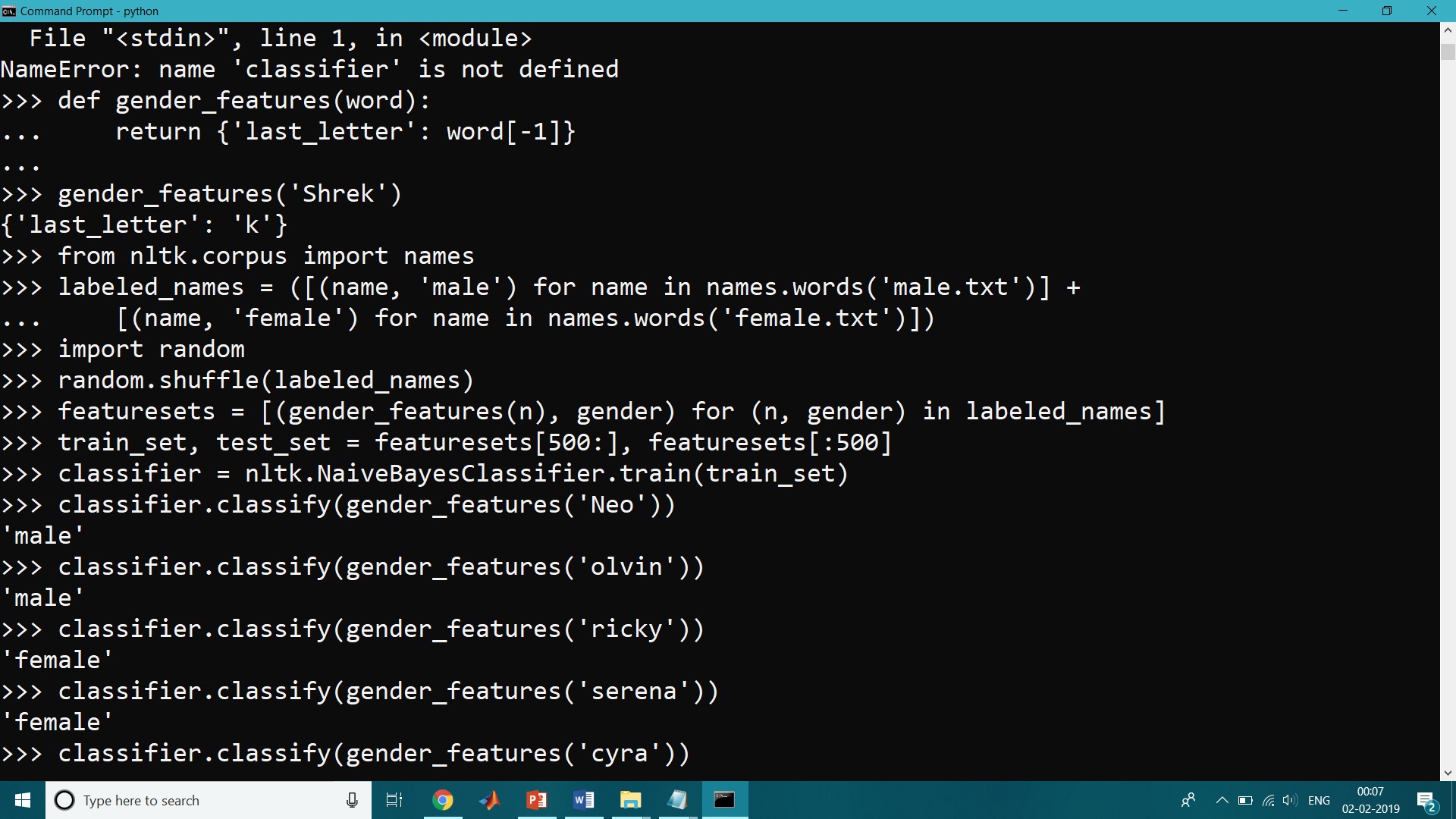
>>> def gender_features(word):

...     return {'last_letter': word[-1]}

>>> gender_features('Shrek')

{'last_letter': 'k'}
Now that we’ve defined a feature extractor, we need to prepare a list of examples and corresponding class labels.
>>> from nltk.corpus import names

>>> labeled_names = ([(name, 'male') for name in names.words('male.txt')] +

... [(name, 'female') for name in names.words('female.txt')])

>>> import random

>>> random.shuffle(labeled_names)
Next, the feature extractor is using to process the names data and divide the resulting list of feature sets into a training set and a test set. The training set is used to train a new “naive Bayes” classifier.
>>> featuresets = [(gender_features(n), gender) for (n, gender) in labeled_names]

>>> train_set, test_set = featuresets[500:], featuresets[:500]

>>> classifier = nltk.NaiveBayesClassifier.train(train_set)
Let’s just test it out on some names that did not appear in its training data:
>>> classifier.classify(gender_features('Neo'))

'male'

>>> classifier.classify(gender_features('olvin'))

'male'

>>> classifier.classify(gender_features('ricky'))

'female'

>>> classifier.classify(gender_features('serena'))

'female'

>>> classifier.classify(gender_features('cyra'))

'female'

>>> classifier.classify(gender_features('leeta'))

'female'

>>> classifier.classify(gender_features('rock'))

'male'

>>> classifier.classify(gender_features('jack'))

'male'
We can systematically evaluate the classifier on a much larger quantity of unseen data:
>>> print(nltk.classify.accuracy(classifier, test_set))

0.77
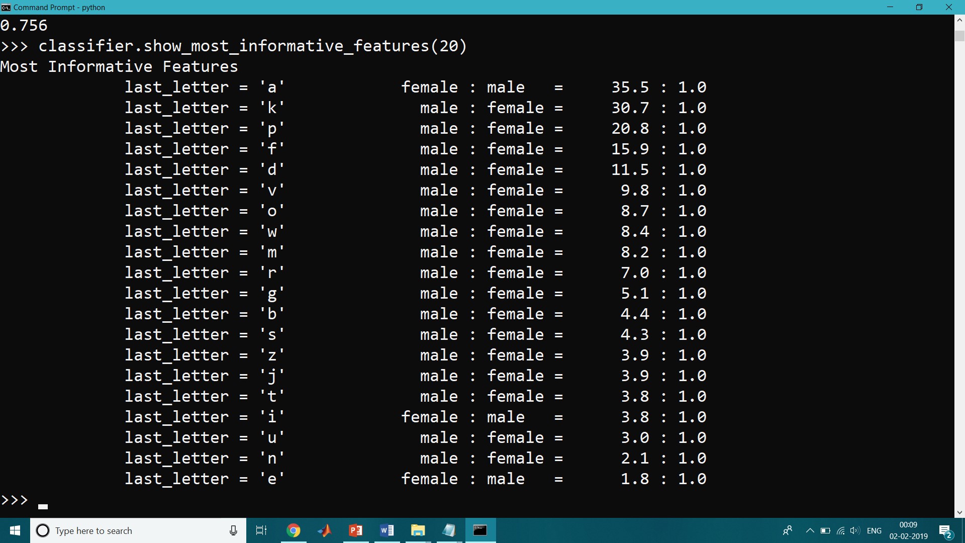
Finally, we can examine the classifier to determine which features it found most effective for distinguishing the names’ genders:
>>> classifier.show_most_informative_features(20)

Most Informative Features

last_letter = 'a'            female : male   =     35.5 : 1.0

last_letter = 'k'              male : female =     30.7 : 1.0

last_letter = 'p'              male : female =     20.8 : 1.0

last_letter = 'f'              male : female =     15.9 : 1.0

last_letter = 'd'              male : female =     11.5 : 1.0

last_letter = 'v'              male : female =      9.8 : 1.0

last_letter = 'o'              male : female =      8.7 : 1.0

last_letter = 'w'              male : female =      8.4 : 1.0

last_letter = 'm'              male : female =      8.2 : 1.0

last_letter = 'r'              male : female =      7.0 : 1.0

last_letter = 'g'              male : female =      5.1 : 1.0

last_letter = 'b'              male : female =      4.4 : 1.0

last_letter = 's'              male : female =      4.3 : 1.0

last_letter = 'z'              male : female =      3.9 : 1.0

last_letter = 'j'              male : female =      3.9 : 1.0

last_letter = 't'              male : female =      3.8 : 1.0

last_letter = 'i'            female : male   =      3.8 : 1.0

last_letter = 'u'              male : female =      3.0 : 1.0

last_letter = 'n'              male : female =      2.1 : 1.0

last_letter = 'e'            female : male   =      1.8 : 1.0
